2 TLSs - Decay in waveguide (non-Markovian regime)

This is an example of 2 two-level systems (TLS1 and TLS2) decaying into the waveguide in the non-Markovian regime (with feedback).

All the examples are in units of the TLS total decay rate, gamma. Hence, in general, gamma=1.

Computes time evolution, population dynamics, and entanglement entropies.

Example plots:

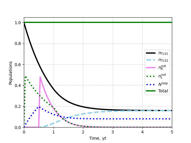
1. TLS population dynamics

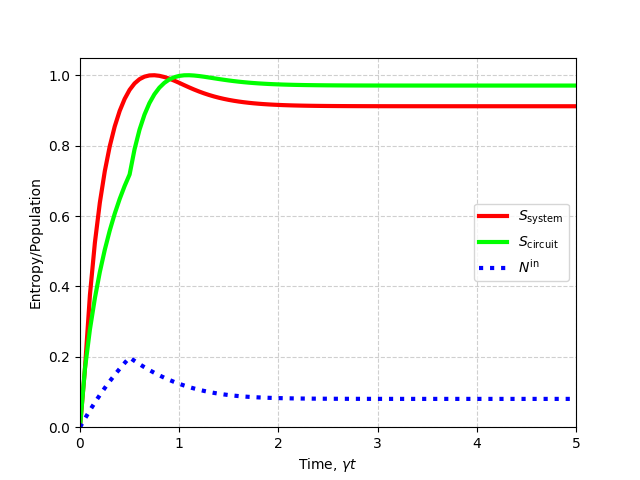
2. Entanglement entropy with the flux

References: Phys. Rev. Research 3, 023030, Arranz-Regidor et. al. (2021)

Imports

import QwaveMPS as qmps
import matplotlib.pyplot as plt
import numpy as np
import time as t

Population dynamics

Choose the simulation parameters

""""Choose the simulation parameters"""
#Choose the bins:
d_t_l=2 #Time right channel bin dimension
d_t_r=2 #Time left channel bin dimension
d_t_total=np.array([d_t_l,d_t_r])

d_sys1=2 # first tls bin dimension
d_sys2=2 # second tls bin dimension
d_sys_total=np.array([d_sys1, d_sys2]) #total system bin dimension

#Choose the coupling:
gamma_l1,gamma_r1=qmps.coupling('symmetrical',gamma=1)
gamma_l2,gamma_r2=qmps.coupling('symmetrical',gamma=1)

#Define input parameters
#Need to define the delay time tau and phase
input_params = qmps.parameters.InputParams(
    delta_t=0.05,
    tmax = 5,
    d_sys_total=d_sys_total,
    d_t_total=d_t_total,
    gamma_l=gamma_l1,
    gamma_r = gamma_r1,
    gamma_l2 = gamma_l2,
    gamma_r2 = gamma_r2,
    bond_max=8,
    phase=np.pi,
    tau=0.5 # Time delay between the two TLS's
)


#Make a tlist for plots:
tmax=input_params.tmax
delta_t=input_params.delta_t
tlist=np.arange(0,tmax+delta_t,delta_t)

Choose the initial state and Hamiltonian

Choose the initial state of each of the TLSs, the waveguide initial state, and the non-Markovian Hamiltonian for 2 TLSs

""" Choose the initial state"""
# Initial system state is an outer product of the two system states
tls1_initial_state=qmps.states.tls_excited()
tls2_initial_state= qmps.states.tls_ground()
sys_initial_state=np.kron(tls1_initial_state,tls2_initial_state)

#We can start with one excited and one ground, both excited, both ground,
# or with an entangled state like the following one
# sys_initial_state=1/np.sqrt(2)*(np.kron(tls1_initial_state,tls2_initial_state)+np.kron(tls2_initial_state,tls1_initial_state))

wg_initial_state = qmps.states.vacuum(tmax,input_params)

start_time=t.time()

"""Choose the Hamiltonian"""
hm=qmps.hamiltonian_2tls_nmar(input_params)

Calculate the time evolution

Time evolution calculation in the non-Markovian regime

""" Time evolution of the system"""
bins = qmps.t_evol_nmar(hm,sys_initial_state,wg_initial_state,input_params)

Choose and calculate the observables

""" Calculate population dynamics"""
# Create system operators as outer products of individual TLS Hilbert spaces
tls1_pop_op = np.kron(qmps.tls_pop(), np.eye(d_sys2))
tls2_pop_op = np.kron(np.eye(d_sys1), qmps.tls_pop())

# Create photonic flux operators in each direction
photon_flux_l_op = qmps.b_pop_l(input_params)
photon_flux_r_op = qmps.b_pop_r(input_params)
photon_flux_ops = [photon_flux_l_op, photon_flux_r_op]

# Calculate time dependent TLS populations, and fluxes into/out of feedback loop
tls_pops = qmps.single_time_expectation(bins.system_states, [tls1_pop_op, tls2_pop_op])
photon_fluxes_out = qmps.single_time_expectation(bins.output_field_states, photon_flux_ops)
photon_fluxes_loop = qmps.single_time_expectation(bins.loop_field_states, photon_flux_ops)

# Use helper function to integrate over the flux into the loop in windows to get loop population
loop_sum_l = qmps.loop_integrated_statistics(photon_fluxes_loop[0], input_params)
loop_sum_r = qmps.loop_integrated_statistics(photon_fluxes_loop[1], input_params)

# Sum the population of the 2 TLS's, the integral of the flux out of the total system, and the population
#  in the loop between the TLS's.
total_quanta = np.sum(tls_pops, axis=0) + np.cumsum(np.sum(photon_fluxes_out, axis=0))*delta_t\
      + loop_sum_l + loop_sum_r

print("--- %s seconds ---" %(t.time() - start_time))

--- 0.6429874897003174 seconds ---

Plot the results

plt.plot(tlist, np.real(tls_pops[0]), linewidth=3, color='k', linestyle='-',label=r'$n_{\rm TLS1}$')
plt.plot(tlist, np.real(tls_pops[1]), linewidth=3, color='skyblue', linestyle='--',label=r'$n_{\rm TLS2}$')
# Graphing the fluxes out this time
plt.plot(tlist, np.real(photon_fluxes_out[1]), linewidth=3, color='violet',linestyle='-',label=r'$n^{\rm out}_{R}$')
plt.plot(tlist, np.real(photon_fluxes_out[0]), linewidth=3, color='green',linestyle=':',label=r'$n^{\rm out}_{L}$')
plt.plot(tlist, np.real(loop_sum_l + loop_sum_r), linewidth=3,color='b',linestyle=':',label=r'$N^{\rm loop}$')
plt.plot(tlist, np.real(total_quanta), linewidth=3, color='g',linestyle='-',label='Total')
plt.legend()
plt.xlabel(r'Time, $\gamma t$')
plt.ylabel('Populations')
plt.grid(True, linestyle='--', alpha=0.6)
plt.ylim([0.,1.05])
plt.xlim([0.,tmax])
plt.show()

Entanglement entropy

Calculate the entanglement entropy

#To track computational time
start_time=t.time()

"""Calculate entanglement entropy"""
# Use given function with the schmidt coefficients saved from the simulation in the Bins object
# Determine the entanglement entropy between the 2 TLS's and the whole waveguide
ent_s=qmps.entanglement(bins.schmidt)

# Determine the entanglement entropy between the 2 TLS's with the section of the waveguide
# between them and with the rest of the waveguide.
ent_s_tau=qmps.entanglement(bins.schmidt_tau)


print("Entanglement--- %s seconds ---" %(t.time() - start_time))

Entanglement--- 0.002596616744995117 seconds ---

Plot the results

plt.plot(tlist,np.real(ent_s),linewidth = 3,color = 'r',linestyle='-',label=r'$S_{\rm system}$')
plt.plot(tlist,np.real(ent_s_tau),linewidth = 3,color = 'lime',linestyle='-',label=r'$S_{\rm circuit}$')
plt.plot(tlist,np.real(loop_sum_l + loop_sum_r),linewidth = 3,color = 'b',linestyle=':',label=r'$N^{\rm in}$')
plt.legend()
plt.xlabel(r'Time, $\gamma t$')
plt.ylabel('Entropy/Population')
plt.grid(True, linestyle='--', alpha=0.6)
plt.ylim([0.,1.05])
plt.xlim([0.,tmax])
plt.show()