Theory

Waveguide QED

Waveguide quantum electrodynamics (QED) systems study quasi one-dimensional quantum systems where atoms or quantum emitters couple to a continuum of quantized field modes. These systems show new phenomena that are unique to the waveguide geometry, such as significant non-Markovian or delayed feedback effects, which can lead to the emission and reabsorption of photons by the quantum emitters, or the ability to couple to chiral emitters, breaking the local symmetry of the problem by emitting photons only in one waveguide direction for a better flow of the quantum information.

The general form of the Hamiltonian is,

\[ H = H_{\rm sys} + H_{\rm W} + H_{\rm I},\]

where \(H_{\rm sys}\) corresponds to the emiiters Hamiltonian, \(H_{\rm W}\) is the waveguide Hamiltonian, and \(H_{\rm I}\) represents the interaction between the emitters and the waveguide. Although system and interaction terms will change form depending on the specific problem, the waveguide Hamiltonian can generally be expressed as,

\[H_{\rm W} = \sum_{\alpha=L,R} \int_{\mathcal{B}} d\omega \omega b_\alpha^\dagger (\omega)b_\alpha(\omega)\]

where \(b_\alpha^\dagger (\omega)\) and \(b_\alpha(\omega)\) are the creation and annihilation bosonic operators for the right- and left-moving photons, and \(\mathcal{B}\) is the relevant bandwidth of interest around the resonance frequency \(\omega_0\), in the rotating-wave approximation.

To solve these complex problems, many theories make use of approximations, such as the Markovian approximation, which results in valuable information being lost. In this project, we give a tool to solve waveguide QED problems using matrix product states (MPS), which allows us to solve these systems without making some of the usual approximations [1,2,3].

For this, we need to discretize the waveguide in time into the so-called ``time bins’’ and write the discretized Hamiltonian in time using the boson noise operators,

\[\Delta B_{R/L} ^{(\dagger)} = \int_{t_k}^{t_{k+1}} dt' b_{R/L}^{(\dagger)}(t')\]

that create/annihilate a photon in a time bin with a commutation relation \(\left[ \Delta B_{R/L}(t_k), \Delta B_{R/L}^\dagger(t_{k'}) \right] = \Delta t \delta_{k,k'} \delta_{R,L}\). With this, we create a new basis,

\[\ket{i^\alpha_k} = \frac{(\Delta B_\alpha^\dagger (t_k))^{i^\alpha_k}}{\sqrt{i^\alpha_k ! (\Delta t)^{i^\alpha_k}}} \ket{\rm vac},\]

and write the time evolution operator for each time step,

\[ U(t_{k+1},t_k) = \exp{ \left( -i \int_{t_k}^{t_{k+1}} dt' H(t')\right)}. \]

Then, the initial state is written in terms of MPS, and the time evolution operator is transformed to a matrix product operator (MPO) to be able to evolve the system one time step at a time.

Matrix Product States

Singular value decomposition

Matrix product states is an approach based on one-dimensional tensor network theories [1,4]. The MPS algorithm relies on the Schmidt or singular value decomposition (SVD) of a quantum system, which considers the bipartition state of the system as a tensor product. The SVD decomposition of a tensor \(M\) is,

\[M = U S V^\dagger,\]

where \(S\) is a diagonal matrix containing the Schmidt coefficients in descending order, \(U\) is a left-normalized tensor, and \(V\) is a right-normalized one. Afterwards, one of the side tensors can be contracted with the tensor containing the Schmidt coefficients. This receives the name of the orthogonality center (OC) and carries the system’s information. Thus, we end up with 2 new tensors written as a tensor product. To better understand the process, this can be represented diagrammatically,

Here, the vertical lines correspond to the physical dimensions of the system, while the horizontal ones represent the bond or virtual extra dimensions generated when performing the SVDs.

Matrix product states

By iterating this process, we can decompose the Hilbert space into a tensor product of smaller subspaces until we get the following general MPS expression for a waveguide QED system,

\[\ket{\psi}=\sum_{i_s i_1...i_N} A_{a_1}^{i_s}A_{a_1,a_2}^{i_1} ... A_{a_{N-1},a_{N}}^{i_{N-1}}A_{a_{N}}^{i_{N}}\ket{i_s, i_1,...,i_N},\]

where the first term represents the system (or quantum emitter) part, and the remaining \(N\) terms represent the waveguide discretized in time. Here, each tensor can be represented as a ‘bin’ which corresponds to the boxes in the diagrammatic representation. This gives the possibility of at least \(N\) photons in the waveguide.

In this diagram, \(i_s i_1...i_N\) represent the physical indices of the MPS.

As an example, let us say that our system contains a single TLS that starts excited, the TLS bin is represented by,

def tls_excited(d_sys1:int=2, bond0:int=1) -> np.ndarray:
    i_s = np.zeros([bond0,d_sys1,bond0],dtype=complex) 
    i_s[:,1,:]=1.
    return i_s

And if the waveguide field starts in vacuum, each time bin will follow,

def wg_ground(d_t:int, bond0:int=1) -> np.ndarray:
    i= np.zeros([bond0,d_t,bond0],dtype=complex) 
    i[:,0,:]=1.
    return i

with the total field being a tensor product of these time bins.

Matrix product operators

An operator can be seen as a projector which projects one physical index \(i\) to another \(j\) with some coefficients \(O^{ij}\). Thus, MPOs have two physical indices per site. The main advantage is that the whole state does not need to be computed when an operator is applied. Only the sites involved in the operation are computed, highly reducing the computational cost of the operation.

For example, an MPO operating on a single site can be represented as,

where \(i_1\) and \(j_1\) are the labels for the physical indices of the corresponding bra and ket. This can be directly applied on the MPS corresponding MPS bin.

As an example, we can implement a noise operator as an MPO following,

def delta_b(delta_t:float, d_t:int=2) -> np.ndarray:     
    return np.sqrt(delta_t) * np.diag(np.sqrt(np.arange(1, d_t, dtype=complex)), 1)

where \(d_t\) is 2 by default to allow one photon per time bin.

Time evolution

The evolution of the system is performed by applying the time evolution operator on the relevant parts of the MPS at each time step. In the Markovian regime or when we do not have feedback effects, this is usually on the system bin and the present time bin. For example, at a time \(t_k\),

where in this case the evolution operator is a 2-site MPO. However, in cases with feedback effects in the non-Markovian regime, we will have to consider also the feedback bins. For example, if we have a feedback bin, \(i_\tau\), the time evolution operator is now a 3-site MPO,

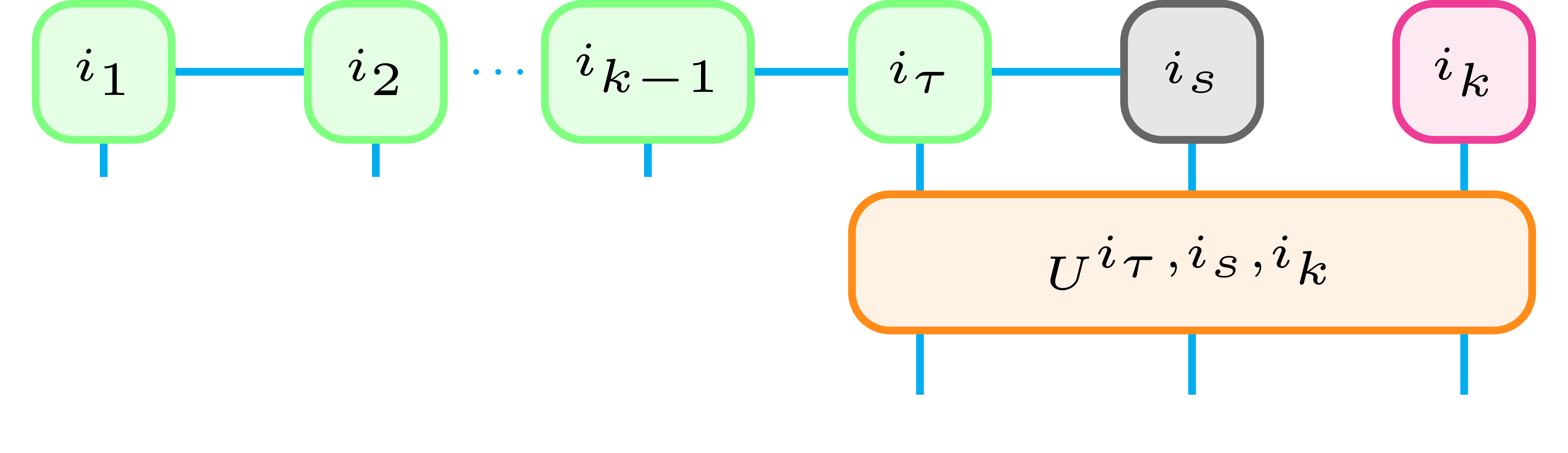
where we have first brought the feedback time bin next to the system bin \(i_s\) and the present time bin \(i_k\) by applying a swap operator, in order to then apply \(U\) only in three sites.

In all the cases, after applying the time evolution operator, the state is again decomposed, performing SVD to recover the MPS shape of each bin. By iterating this process, the evolution of the system is calculated.

References

[1] Hannes Pichler and Peter Zoller, “Photonic circuits with time delays and quantum feedback,” Phys. Rev. Lett. 116, 093601 (2016).

[2] Hannes Pichler, Soonwon Choi, Peter Zoller, and Mikhail D. Lukin, “Universal photonic quantum computation via time-delayed feedback,” Proceedings of the National Academy of Sciences 114, 11362–11367 (2017).

[3] Sofia Arranz Regidor, Gavin Crowder, Howard Carmichael, and Stephen Hughes, “Modeling quantum light-matter interactions in waveguide QED with retardation, nonlinear interactions, and a time-delayed feedback: Matrix product states versus a space-discretized waveguide model,” Phys. Rev. Res. 3, 023030 (2021).

[3] R. Orús, A practical introduction to tensor networks: Matrix product states and projected entangled pair states, Annals of Physics 349, 117 (2014)