2 TLSs - Decay in waveguide (Markovian regime)

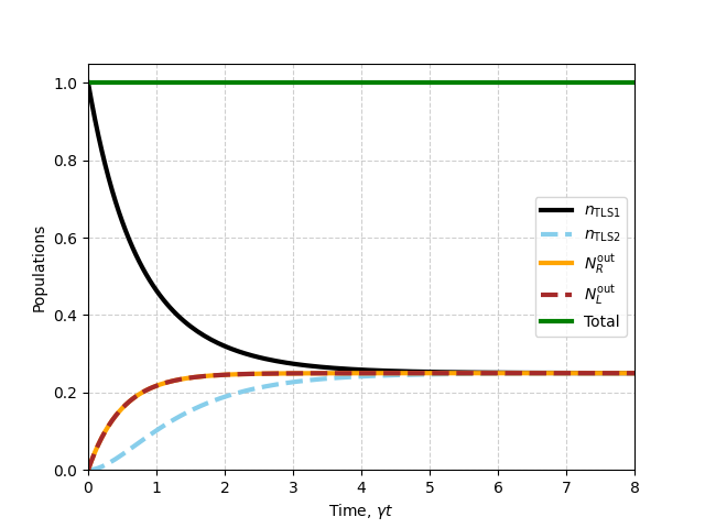
This is an example of 2 two-level systems (TLS1 and TLS2) decaying into the waveguide in the Markovian regime.

All the examples are in units of the TLS total decay rate, gamma. Hence, in general, gamma=1.

Computes time evolution, population dynamics, and the entanglement entropy.

Example plots:

1. TLS population dynamics

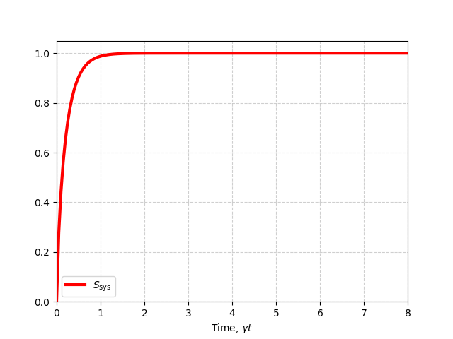
2. Entanglement entropy

Imports

import QwaveMPS as qmps
import matplotlib.pyplot as plt
import numpy as np
import time as t

Population dynamics

Choose the simulation parameters

""""Choose the simulation parameters"""
#Choose the Hilbert space sizes:
d_t_l=2 #Time right channel bin dimension
d_t_r=2 #Time left channel bin dimension
d_t_total=np.array([d_t_l,d_t_r])

d_sys1=2 # first tls bin dimension
d_sys2=2 # second tls bin dimension
d_sys_total=np.array([d_sys1, d_sys2]) #total system bin dimension

#Choose the coupling for each TLS:
gamma_l1,gamma_r1=qmps.coupling('symmetrical',gamma=1)
gamma_l2,gamma_r2=qmps.coupling('symmetrical',gamma=1)

#Define input parameters
input_params = qmps.parameters.InputParams(
    delta_t=0.05, # Simulation time step
    tmax = 8, # Maximum simulation time
    d_sys_total=d_sys_total,
    d_t_total=d_t_total,

    # Couplings
    gamma_l=gamma_l1,
    gamma_r = gamma_r1,
    gamma_l2 = gamma_l2,
    gamma_r2 = gamma_r2,

    bond_max=4, # Maximum MPS bond dimension, sets truncation of entanglement
    phase=np.pi # Phase of interaction between the 2 TLS's
)


#Make a tlist for plots:
tmax=input_params.tmax
delta_t=input_params.delta_t
tlist=np.arange(0,tmax+delta_t/2,delta_t)

Choose the initial state and Hamiltonian

Choose the initial state of each of the TLSs, the waveguide initial state, and the Markovian Hamiltonian for 2 TLSs

""" Choose the initial state"""
#Starting with the firt TLS excited and the second in ground state
tls1_initial_state=qmps.states.tls_excited()
tls2_initial_state= qmps.states.tls_ground()

# The total system initial state is the outer product of the two TLS's states
sys_initial_state=np.kron(tls1_initial_state,tls2_initial_state)

#If starting with an entangled initial state
# sys_initial_state=1/np.sqrt(2)*(np.kron(tls1_initial_state,tls2_initial_state) + np.kron(tls2_initial_state,tls1_initial_state))

wg_initial_state = qmps.states.vacuum(tmax, input_params)
# wg_initial_state = None # Another way to set the same initial state


"""Choose the Hamiltonian"""
hm=qmps.hamiltonian_2tls_mar(input_params)

#To track computational time
start_time=t.time()

Calculate the time evolution

Time evolution calculation in the Markovian regime

"""Calculate time evolution of the system"""
bins = qmps.t_evol_mar(hm,sys_initial_state,wg_initial_state,input_params)

Choose and calculate the observables

"""Define relevant observable operators"""
# System operators are outerproducts of the two TLS Hilbert spaces
pop_tls1_op = np.kron(qmps.tls_pop(), np.eye(d_sys2))
pop_tls2_op = np.kron(np.eye(d_sys1), qmps.tls_pop())

# Left and right population/flux operators for the output field
flux_l_op = qmps.b_dag_l(input_params) @ qmps.b_l(input_params)
flux_r_op = qmps.b_dag_r(input_params) @ qmps.b_r(input_params)

"""Calculate population dynamics"""
tls_pops = qmps.single_time_expectation(bins.system_states, [pop_tls1_op, pop_tls2_op])
fluxes = qmps.single_time_expectation(bins.output_field_states, [flux_l_op, flux_r_op])

# Integrating over outgoing flux and sum over flux directions/TLS populations
total_quanta = np.sum(tls_pops,axis=0) + np.cumsum(np.sum(fluxes,axis=0)) * delta_t
# An equivalent formulation
#total_quanta = tls_pops[0] + tls_pops[1] + np.cumsum(fluxes[0] + fluxes[1]) * delta_t

print("--- %s seconds ---" %(t.time() - start_time))

--- 0.12050056457519531 seconds ---

Plot the results

plt.plot(tlist,np.real(tls_pops[0]),linewidth = 3, color = 'k',linestyle='-',label=r'$n_{\rm TLS1}$')
plt.plot(tlist,np.real(tls_pops[1]),linewidth = 3, color = 'skyblue',linestyle='--',label=r'$n_{\rm TLS2}$')
plt.plot(tlist,np.real(np.cumsum(fluxes[0])*delta_t),linewidth = 3,color = 'orange',linestyle='-',label=r'$N_R^{\rm out}$') # Net flux out right
plt.plot(tlist,np.real(np.cumsum(fluxes[1])*delta_t),linewidth = 3,color = 'brown',linestyle='--',label=r'$N_L^{\rm out}$') # Net flux out left
plt.plot(tlist,np.real(total_quanta),linewidth = 3,color = 'g',linestyle='-',label='Total')
plt.legend()
plt.xlabel(r'Time, $\gamma t$')
plt.ylabel('Populations')
plt.grid(True, linestyle='--', alpha=0.6)
plt.ylim([0.,1.05])
plt.xlim([0.,tmax])
plt.show()

Entanglement entropy

Calculate the entanglement entropy

#To track computational time
start_time=t.time()

"""Calculate entanglement entropy"""
# Use given function with the schmidt coefficients saved from the simulation in the Bins object
ent_s=qmps.entanglement(bins.schmidt)

print("Entanglement--- %s seconds ---" %(t.time() - start_time))

Entanglement--- 0.0020253658294677734 seconds ---

Plot the results

plt.plot(tlist,np.real(ent_s),linewidth = 3,color = 'r',linestyle='-',label=r'$S_{\rm sys}$')
plt.legend()
plt.xlabel(r'Time, $\gamma t$')
plt.grid(True, linestyle='--', alpha=0.6)
plt.ylim([0.,1.05])
plt.xlim([0.,tmax])
plt.show()