1 TLS - Decay in semi-infinite waveguide

This is an example of a single two-level system (TLS) decaying into a semi-infinite waveguide with a side mirror. This is calculated in the non-Markovian regime with a delay time tau, that in this case is the roundtrip time of the feedback loop (back and forth from the mirror), and a phase that can be constructive or destructive.

All the examples are in units of the TLS total decay rate, gamma. Hence, in general, gamma=1.

It covers two cases:

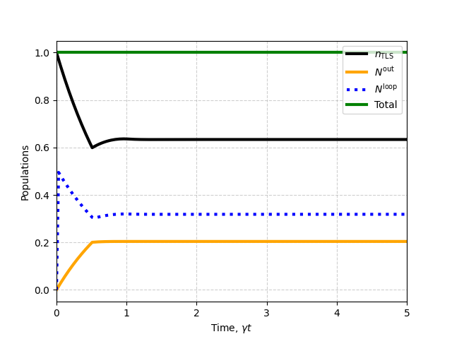
1. Example with constructive feedback (tau=0.5, phase=\(\pi\))

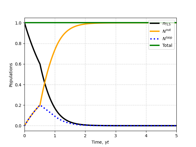
2. Example with destructive feedback (tau=0.5, phase=0)

References: Phys. Rev. Research 3, 023030, Arranz-Regidor et. al. (2021)

Imports

import QwaveMPS as qmps
import matplotlib.pyplot as plt
import numpy as np
import time as t

Example with constructive feedback

Choose the simulation parameters

Choose a constructive feedback phase, e.g. phase=\(\pi\)

#Choose the bins:
d_sys1=2 # tls bin dimension
d_sys_total=np.array([d_sys1]) #total system bin (in this case only 1 tls)

d_t=2 #time bin dimension of one channel
d_t_total=np.array([d_t]) #single channel for mirror case

#Choose the coupling
gamma_l,gamma_r=qmps.coupling('symmetrical',gamma=1)

#Define input parameters
input_params = qmps.parameters.InputParams(
    delta_t=0.03, # simulation time step
    tmax = 5, # simulation total time length
    d_sys_total=d_sys_total,
    d_t_total=d_t_total,
    gamma_l=gamma_l,
    gamma_r = gamma_r,
    bond_max=4, #simulation maximum MPS bond dimension, truncates entanglement information
    tau=0.5, # Roundtrip feedback time
    phase=np.pi
)


#Make a tlist for plots:
tmax=input_params.tmax
delta_t=input_params.delta_t
tlist=np.arange(0,tmax+delta_t/2,delta_t)

Choose the initial state and Hamiltonian

""" Choose the initial state"""
sys_initial_state=qmps.states.tls_excited()

#wg_initial_state = qmps.states.vacuum(tmax,input_params)
wg_initial_state = None # Showing that None is the vacuum state

#To track computational time
start_time=t.time()

"""Choose the Hamiltonian"""
Hm=qmps.hamiltonian_1tls_feedback(input_params)

Calculate the time evolution

Time evolution calculation in the non-Markovian regime:

""" Time evolution of the system"""
bins = qmps.t_evol_nmar(Hm,sys_initial_state,wg_initial_state,input_params)

Choose and calculate the observables

""" Calculate population dynamics"""
# Use single channel bosonic operators, chiral waveguide Hilbert space
# This is because len(d_t_total) == 1
flux_op = qmps.b_pop(input_params)

# Another way to define the same op
#flux_op = qmps.b_dag(input_params) @ qmps.b(input_params)

tls_pops = qmps.single_time_expectation(bins.system_states, qmps.tls_pop())

# Calculate the flux out of the system (exiting the loop)
transmitted_flux = qmps.single_time_expectation(bins.output_field_states, flux_op)

# If we want to calculate the net transmitted quanta have to integrate the flux
net_transmitted_quanta = np.cumsum(transmitted_flux) * delta_t

# Calculate the flux into the feedback loop
loop_flux = qmps.single_time_expectation(bins.loop_field_states, flux_op)

# Helper function to integrate an operator over the feedback loop time points
# Here returns a time dependent function (list) of the total excitation number
#  in the feedback loop
loop_sum = qmps.loop_integrated_statistics(loop_flux, input_params)

total_quanta = tls_pops + loop_sum + np.cumsum(transmitted_flux)*delta_t

print("--- %s seconds ---" %(t.time() - start_time))

--- 0.7771546840667725 seconds ---

Plot the results

plt.plot(tlist,np.real(tls_pops),linewidth = 3, color = 'k',linestyle='-',label=r'$n_{\rm TLS}$')
plt.plot(tlist,np.real(net_transmitted_quanta),linewidth = 3,color = 'orange',linestyle='-',label=r'$N^{\rm out}$')
plt.plot(tlist,np.real(loop_flux),linewidth = 3,color = 'b',linestyle=':',label=r'$N^{\rm loop}$')
plt.plot(tlist,np.real(total_quanta),linewidth = 3,color = 'g',linestyle='-',label='Total')
plt.legend(loc='upper right')
plt.grid(True, linestyle='--', alpha=0.6)
plt.xlim([0.,tmax])
plt.xlabel(r'Time, $\gamma t$')
plt.ylabel('Populations')
plt.show()

Example with destructive feedback

Update the simulation parameters

Choose a destructive feedback phase, e.g. phase=0

#update it in the input parameters
input_params.phase=0

Update Hamiltonian

"""Choose the Hamiltonian"""
hm=qmps.hamiltonian_1tls_feedback(input_params)

Calculate the time evolution

""" Time evolution of the system"""
bins = qmps.t_evol_nmar(hm,sys_initial_state,wg_initial_state,input_params)

Calculate the observables

""" Calculate population dynamics"""
tls_pops = qmps.single_time_expectation(bins.system_states, qmps.tls_pop())
transmitted_flux = qmps.single_time_expectation(bins.output_field_states, flux_op)
loop_flux = qmps.single_time_expectation(bins.loop_field_states, flux_op)

"""Integrate again over the total quanta in the feedback loop"""
loop_sum = qmps.loop_integrated_statistics(loop_flux, input_params)
new_transmitted_flux = np.cumsum(transmitted_flux) * delta_t
total_quanta = tls_pops + loop_sum + np.cumsum(transmitted_flux)*delta_t

Plot the results

plt.plot(tlist,np.real(tls_pops),linewidth = 3, color = 'k',linestyle='-',label=r'$n_{\rm TLS}$')
plt.plot(tlist,np.real(new_transmitted_flux),linewidth = 3,color = 'orange',linestyle='-',label=r'$N^{\rm out}$')
plt.plot(tlist,np.real(loop_sum),linewidth = 3,color = 'b',linestyle=':',label=r'$N^{\rm loop}$')
plt.plot(tlist,np.real(total_quanta),linewidth = 3,color = 'g',linestyle='-',label='Total')
plt.legend(loc='upper right')
plt.xlabel(r'Time, $\gamma t$')
plt.ylabel('Populations')
plt.grid(True, linestyle='--', alpha=0.6)
plt.xlim([0.,tmax])
plt.show()