1 TLS - Drive with Fock-state pulse

This is an example of a single two-level system (TLS) interacting with a 1-photon and 2-photon Fock state pulse.

All the examples are in units of the TLS total decay rate, gamma. Hence, in general, gamma=1.

It covers two cases:

1. Example with a 1-photon tophat pulse

2. Example with a 2-photon gaussian pulse

Computes time evolution, population dynamics, and first and second-order correlations (for the 2 photon case), with example plots of the populations for both cases.

References: Phys. Rev. Research 7, 023295 , Arranz-Regidor et. al. (2025)

Imports

import QwaveMPS as qmps
import matplotlib.pyplot as plt
import numpy as np
import time as t

1 photon Tophat Pulse

Choose the simulation parameters

""""Choose the simulation parameters"""
#Choose the bin dimensions
# Here setting to 2 to accommodate a 1 photon space:
d_t_l=2 #Time right channel bin dimension
d_t_r=2 #Time left channel bin dimension
d_t_total=np.array([d_t_l,d_t_r])

d_sys1=2 # tls bin dimension
d_sys_total=np.array([d_sys1]) #total system bin (in this case only 1 tls)

#Choose the coupling:
gamma_l,gamma_r=qmps.coupling('symmetrical',gamma=1)

#Define input parameters
input_params = qmps.parameters.InputParams(
    delta_t=0.05,
    tmax = 8,
    d_sys_total=d_sys_total,
    d_t_total=d_t_total,
    gamma_l=gamma_l,
    gamma_r = gamma_r,
    bond_max=4
)

#Make a tlist for plots:
tmax=input_params.tmax
delta_t=input_params.delta_t
tlist=np.arange(0,tmax+delta_t,delta_t)

Choose the initial state and Hamiltonian

In this case, we need to also specify the pulse parameters that will go in the photonic part of the initial state

""" Choose the initial state and tophat pulse parameters"""
sys_initial_state=qmps.states.tls_ground()

# Pulse parameters por a 1-photon tophat pulse
pulse_time = 1 #length of the pulse in time units of gamma
photon_num = 1 #number of photons

#pulse envelope shape
pulse_env=qmps.states.tophat_envelope(pulse_time, input_params)

# Create the pulse envelope
wg_initial_state = qmps.states.fock_pulse(pulse_env,pulse_time,photon_num, input_params, direction='R')

# Multiple pulses may be appended in the usual list appending way
#wg_initial_state += qmps.states.fock_pulse(pulse_env,pulse_time,photon_num, input_params, direction='L')

"""Choose the Hamiltonian"""
Hm=qmps.hamiltonian_1tls(input_params)

#To track computational time of populations
start_time=t.time()

Calculate the time evolution

Time evolution calculation in the Markovian regime

"""Calculate time evolution of the system"""

bins = qmps.t_evol_mar(Hm,sys_initial_state,wg_initial_state,input_params)

Calculate the population dynamics

"""Calculate population dynamics"""
# Photonic operators
left_flux_op = qmps.b_dag_l(input_params) @ qmps.b_l(input_params)
right_flux_op = qmps.b_dag_r(input_params) @ qmps.b_r(input_params)
photon_flux_ops = [left_flux_op, right_flux_op]

tls_pop = qmps.single_time_expectation(bins.system_states, qmps.tls_pop())
photon_fluxes = qmps.single_time_expectation(bins.output_field_states, photon_flux_ops)
flux_in = qmps.single_time_expectation(bins.input_field_states, photon_flux_ops)

# Calculate total quanta that has entered the system, tls population + net flux out
total_quanta = tls_pop + np.cumsum(photon_fluxes[0] + photon_fluxes[1]) * delta_t
print("--- %s seconds ---" %(t.time() - start_time))

--- 0.12199044227600098 seconds ---

Plot the results

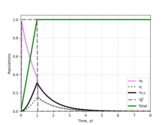
plt.plot(tlist,np.real(photon_fluxes[1]),linewidth = 3,color = 'violet',linestyle='-',label=r'$n_{R}$') # Photon flux transmitted to the right channel
plt.plot(tlist,np.real(photon_fluxes[0]),linewidth = 3,color = 'green',linestyle=':',label=r'$n_{L}$') # Photon flux reflected to the left channel
plt.plot(tlist,np.real(tls_pop),linewidth = 3, color = 'k',linestyle='-',label=r'$n_{TLS}$') # TLS population
plt.plot(tlist,np.real(flux_in[1]),linewidth = 3, color = 'grey',linestyle='--',label=r'$n_{R}^{\rm in}$') # Photon flux in from right
plt.plot(tlist,np.real(total_quanta),linewidth = 3,color = 'g',linestyle='-',label='Total') # Conservation check (for one excitation it should be 1)
plt.legend()
plt.xlabel(r'Time, $\gamma t$')
plt.ylabel('Populations')
plt.grid(True, linestyle='--', alpha=0.6)
plt.ylim([0.,1.05])
plt.xlim([0.,tmax])
plt.show()

Calculate the two-time correlations

In this case, we calculate only the first-order correlation, the second-order correlation is 0 at all times since there is only one photon involved.

Here, we append the operators for each correlation we want to calculate, hence, they can be calculated in same call for faster performance with use of identity operators

"""Calculate correlations """
#To track computational time of g1
start_time=t.time()

# Construct list of ops with the structure <A(t)B(t+t')>
# Much faster to calculate using a list and a single correlation_2op_2t() function call
# than three separate calls
a_op_list = []; b_op_list = []
b_dag_l = qmps.b_dag_l(input_params); b_l = qmps.b_l(input_params)
b_dag_r = qmps.b_dag_r(input_params); b_r = qmps.b_r(input_params)

# Add op <a_R^\dag(t) a_R(t+t')>
a_op_list.append(b_dag_r)
b_op_list.append(b_r)

# Add op <a_L^\dag(t) a_L(t+t')>
a_op_list.append(b_dag_l)
b_op_list.append(b_l)

# Add op <a_L^\dag(t) a_R(t+t')>
a_op_list.append(b_dag_l)
b_op_list.append(b_r)


g1_correlations, correlation_tlist = qmps.correlation_2op_2t(bins.correlation_bins, a_op_list, b_op_list, input_params)

print("G1 correl--- %s seconds ---" %(t.time() - start_time))

Correlation Calculation Completion:
0.0 %
5.0 %
10.1 %
15.1 %
20.1 %
25.2 %
30.2 %
35.2 %
40.3 %
45.3 %
50.3 %
55.3 %
60.4 %
65.4 %
70.4 %
75.5 %
80.5 %
85.5 %
90.6 %
95.6 %
G1 correl--- 6.460116624832153 seconds ---

Plot the results

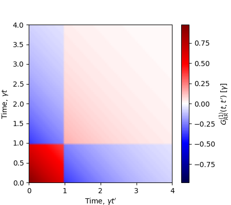
"""Example graphing G1_{RR}"""

X,Y = np.meshgrid(correlation_tlist,correlation_tlist)
# Use a function to transform from t,t' coordinates to t1, t2 so that t2=t+t'
z = np.real(qmps.transform_t_tau_to_t1_t2(g1_correlations[0]))
absMax = np.abs(z).max()


fig, ax = plt.subplots(figsize=(4.5, 4))
cf = ax.pcolormesh(X,Y,z,shading='gouraud',cmap='seismic', vmin=-absMax, vmax=absMax,rasterized=True)
cbar = fig.colorbar(cf,ax=ax)

ax.set_ylabel(r'Time, $\gamma t$')
ax.set_xlabel(r'Time, $\gamma t^\prime$')
ax.set_xlim((0,4))
ax.set_ylim((0,4))
cbar.set_label(r'$G^{(1)}_{RR}(t,t^\prime)\ [\gamma]$')
plt.show()


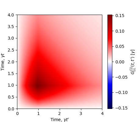
""" Example graphing G1_{LL} """
# Use a function to transform from t,t' coordinates to t1, t2 so that t2=t+t'
z = np.real(qmps.transform_t_tau_to_t1_t2(g1_correlations[1]))
absMax = np.abs(z).max()
fig, ax = plt.subplots(figsize=(4.5, 4))
cf = ax.pcolormesh(X,Y,z,shading='gouraud',cmap='seismic', vmin=-absMax, vmax=absMax,rasterized=True)
cbar = fig.colorbar(cf,ax=ax)

ax.set_ylabel(r'Time, $\gamma t$')
ax.set_xlabel(r'Time, $\gamma t^\prime$')
ax.set_xlim((0,4))
ax.set_ylim((0,4))
cbar.set_label(r'$G^{(1)}_{LL}(t,t^\prime)\ [\gamma]$')
plt.show()

• 
• 

2-photon Gaussian pulse

Update the simulation parameters

""" Update photonic space size input field, simulation length"""
# Set it channel to 3 to accommodate 2 photons
d_t_l=3 #Time right channel bin dimension
d_t_r=3 #Time left channel bin dimension

input_params.d_t_total = np.array([d_t_l,d_t_r])

input_params.tmax=10
tmax=input_params.tmax
tlist=np.arange(0,tmax+delta_t,delta_t)

#We need a higher bond dimension for a 2-photon pulse
input_params.bond_max=8

Update the initial state

sys_initial_state=qmps.states.tls_ground()

# Pulse parameters for a 2-photon gaussian pulse
pulse_time = tmax
photon_num = 2
gaussian_center = 4
gaussian_width = 1

pulse_envelope = qmps.states.gaussian_envelope(pulse_time, input_params, gaussian_width, gaussian_center)
wg_initial_state = qmps.states.fock_pulse(pulse_envelope,pulse_time, photon_num, input_params, direction='R')

start_time=t.time()

Calculate the time evolution

"""Calculate time evolution of the system"""
# Create the Hamiltonian again for this larger Hilbert space
Hm=qmps.hamiltonian_1tls(input_params)
bins = qmps.t_evol_mar(Hm,sys_initial_state,wg_initial_state,input_params)

Calculate the population dynamics

"""Calculate population dynamics"""
photon_flux_ops = [qmps.b_pop_l(input_params), qmps.b_pop_r(input_params)]

# Calculate same time G2 in transmission
same_time_G2_op = qmps.b_dag_r(input_params) @ qmps.b_dag_r(input_params) @ qmps.b_r(input_params) @ qmps.b_r(input_params)

tls_pop = qmps.single_time_expectation(bins.system_states, qmps.tls_pop())
photon_fluxes = qmps.single_time_expectation(bins.output_field_states, photon_flux_ops)
same_time_G2 = qmps.single_time_expectation(bins.output_field_states, same_time_G2_op)

# Act on input states to characterize the input field with bosonic/field operators
flux_in = qmps.single_time_expectation(bins.input_field_states, photon_flux_ops)


total_quanta = tls_pop + np.cumsum(photon_fluxes[0] + photon_fluxes[1]) * delta_t

print("2-photon pop--- %s seconds ---" %(t.time() - start_time))

2-photon pop--- 0.32308220863342285 seconds ---

Plot the results

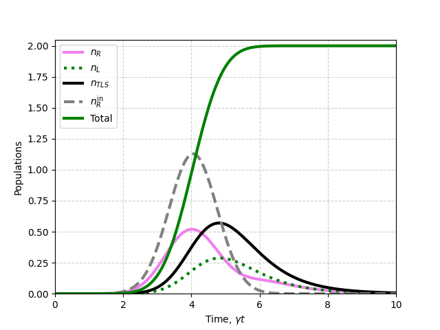
plt.plot(tlist,np.real(photon_fluxes[1]),linewidth = 3,color = 'violet',linestyle='-',label=r'$n_{R}$') # Photons transmitted to the right channel
plt.plot(tlist,np.real(photon_fluxes[0]),linewidth = 3,color = 'green',linestyle=':',label=r'$n_{L}$') # Photons reflected to the left channel
plt.plot(tlist,np.real(tls_pop),linewidth = 3, color = 'k',linestyle='-',label=r'$n_{TLS}$') # TLS population
plt.plot(tlist,np.real(flux_in[1]),linewidth = 3, color = 'grey',linestyle='--',label=r'$n_{R}^{\rm in}$') # Photon flux in from right
plt.plot(tlist,np.real(total_quanta),linewidth = 3,color = 'g',linestyle='-',label='Total') # Conservation check (for one excitation it should be 1)
plt.legend()
plt.xlabel(r'Time, $\gamma t$')
plt.ylabel('Populations')
plt.grid(True, linestyle='--', alpha=0.6)
plt.ylim([0.,2.05])
plt.xlim([0.,tmax])
plt.show()

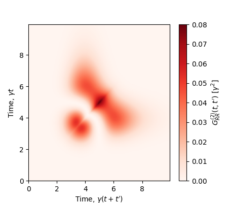
Calculate the two-time correlations

Here, we show how to calculate the second-order correlation which will have values different from 0 since the pulse contains now 2 photons.

#To track computational time of G2
start_time=t.time()

# For speed calculating several at once, but could also calculate all at once
a_op_list = []; b_op_list = []; c_op_list = []; d_op_list = []

# Have to create operators again for this larger space
b_dag_l = qmps.b_dag_l(input_params); b_l = qmps.b_l(input_params)
b_dag_r = qmps.b_dag_r(input_params); b_r = qmps.b_r(input_params)

# Add op <b_R^\dag(t) b_R^\dag(t+t') b_R^(t+t') b_R(t)>
a_op_list.append(b_dag_r)
b_op_list.append(b_dag_r)
c_op_list.append(b_r)
d_op_list.append(b_r)

# Add op <b_L^\dag(t) b_L^\dag(t+t') b_L^(t+t') b_L(t)>
a_op_list.append(b_dag_l)
b_op_list.append(b_dag_l)
c_op_list.append(b_l)
d_op_list.append(b_l)


# Add op <b_R^\dag(t) b_L^\dag(t+t') b_L^(t+t') b_R(t)>
a_op_list.append(b_dag_r)
b_op_list.append(b_dag_l)
c_op_list.append(b_l)
d_op_list.append(b_r)

# Add op <b_L^\dag(t) b_R^\dag(t+t') b_R^(t+t') b_L(t)>
a_op_list.append(b_dag_l)
b_op_list.append(b_dag_r)
c_op_list.append(b_r)
d_op_list.append(b_l)

# Could also consider G1 correlation functions in the same call if we were interested
# For example: <b_R^\dag(t)b_R(t+t')>
a_op_list.append(b_dag_r)
b_op_list.append(b_r)
c_op_list.append(np.eye(input_params.d_t))
d_op_list.append(np.eye(input_params.d_t))

g2_correlations, correlation_tlist = qmps.correlation_4op_2t(bins.correlation_bins, a_op_list, b_op_list, c_op_list, d_op_list, input_params)


print("G2 correl--- %s seconds ---" %(t.time() - start_time))

Correlation Calculation Completion:
0.0 %
5.0 %
10.1 %
15.1 %
20.1 %
25.1 %
30.2 %
35.2 %
40.2 %
45.2 %
50.3 %
55.3 %
60.3 %
65.3 %
70.4 %
75.4 %
80.4 %
85.4 %
90.5 %
95.5 %
G2 correl--- 392.87004494667053 seconds ---

Plot the results

X,Y = np.meshgrid(correlation_tlist,correlation_tlist)


"""Example graphing G2_{RR}"""
# Use a function to transform from t,t' coordinates to t1, t2 so that t2=t+t'
z = np.real(qmps.transform_t_tau_to_t1_t2(g2_correlations[0]))
absMax = np.abs(z).max()

fig, ax = plt.subplots(figsize=(4.5, 4))
cf = ax.pcolormesh(X,Y,z,shading='gouraud',cmap='Reds', vmin=0, vmax=absMax,rasterized=True)
cbar = fig.colorbar(cf,ax=ax)
ax.set_ylabel(r'Time, $\gamma t$')
ax.set_xlabel(r'Time, $\gamma(t+t^\prime)$')
cbar.set_label(r'$G^{(2)}_{RR}(t,t^\prime)\ [\gamma^{2}]$')
plt.show()


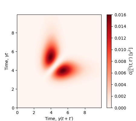
"""Example graphing G2_{LL}"""
z = np.real(qmps.transform_t_tau_to_t1_t2(g2_correlations[1]))
absMax = np.abs(z).max()

fig, ax = plt.subplots(figsize=(4.5, 4))
cf = ax.pcolormesh(X,Y,z,shading='gouraud',cmap='Reds', vmin=0, vmax=absMax,rasterized=True)
cbar = fig.colorbar(cf,ax=ax)
ax.set_ylabel(r'Time, $\gamma t$')
ax.set_xlabel(r'Time, $\gamma(t+t^\prime)$')
cbar.set_label(r'$G^{(2)}_{LL}(t,t^\prime)\ [\gamma^{2}]$')
plt.show()

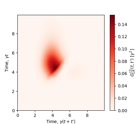
"""Example graphing G2_{LR}"""
# Use a function to transform from t,t' coordinates to t1, t2 so that t2=t+t'
# Since the correlation isn't symmetric w.r.t. t', need both G2_{LR} and G2_{RL}
# Arguments below would be reversed for G2_{RL}
z = np.real(qmps.transform_t_tau_to_t1_t2(g2_correlations[3],g2_correlations[2]))
absMax = np.abs(z).max()

fig, ax = plt.subplots(figsize=(4.5, 4))
cf = ax.pcolormesh(X,Y,z,shading='gouraud',cmap='Reds', vmin=0, vmax=absMax,rasterized=True)
cbar = fig.colorbar(cf,ax=ax)
ax.set_ylabel(r'Time, $\gamma t$')
ax.set_xlabel(r'Time, $\gamma(t+t^\prime)$')
cbar.set_label(r'$G^{(2)}_{LR}(t,t^\prime)\ [\gamma^{2}]$')
plt.show()

• 
• 
•