1 TLS - Decay in infinite waveguide

This is a basic example of a single two-level system (TLS) decaying into an infinite waveguide.

All the examples are in units of the TLS total decay rate, gamma. Hence, in general, gamma=1.

It covers two cases:

1. Symmetrical coupling into the waveguide

2. Chiral coupling, where the TLS is only coupled to the right channel of the waveguide.

Imports

import QwaveMPS as qmps
import matplotlib.pyplot as plt
import numpy as np
import time as t

Symmetrical Solution

Choose the simulation parameters

Setup of the bin size, coupling and input parameters:

• Size of each system bin (d_sys), this is the TLS Hilbert subspace, and the total system bin (d_sys_total) containing all the emitters. For a single TLS, d_sys1=2 and d_sys_total=np.array([d_sys1]).

• Size of the time bins (d_t_total). This contains the field Hilbert subspace at each time step. In this case we allow one photon per time step and per right (d_t_r) and left (d_t_l) channels. Hence, the subspace is d_t_total=np.array([d_t_l,d_t_r])

• Choice of coupling. Here, it is first calculated with symmetrical coupling, gamma_l,gamma_r=qmps.coupling(‘symmetrical’,gamma=1) and then with chiral coupling, gamma_l,gamma_r=qmps.coupling(‘chiral_r’,gamma=1)

• Input parameters (input_params). Define the data parameters that will be used in the calculation:

  • Time step (delta_t)

  • Maximum time (tmax)

  • d_sys_total (as defined above)

  • d_t_total (as defined above)

  • Maximum bond dimension (bond). bond >=d_t_total(number of excitations). Starting with the TLS excited and field in vacuum, 1 excitation enough with bond=4

#Choose the bins:
d_t_l=2 #Time right channel bin dimension
d_t_r=2 #Time left channel bin dimension
d_t_total=np.array([d_t_l,d_t_r]) #Total field bin dimensions

d_sys1=2 # tls bin dimension
d_sys_total=np.array([d_sys1]) #total system bin (in this case only 1 tls)

#Choose the coupling:
gamma_l,gamma_r=qmps.coupling('symmetrical',gamma=1) # same as gamma_l, gamma_r = (0.5,0.5)

#Define input parameters (dataclass)
input_params = qmps.parameters.InputParams(
    delta_t=0.05, # Time step of the simulation
    tmax = 8, # Maximum simulation time
    d_sys_total=d_sys_total,
    d_t_total=d_t_total,
    gamma_l=gamma_l,
    gamma_r = gamma_r,
    bond_max=4 # Maximum bond dimension, simulation parameter that adjusts truncation of entanglement information
)

#Make a tlist for plots:
tmax=input_params.tmax
delta_t=input_params.delta_t
tlist=np.arange(0,tmax+delta_t,delta_t)

Choose the initial state and Hamiltonian

• Choice the system initial state. Here, initially excited.

• Choice of the waveguide initial state. Here, starting in vacuum, and considering that there is vacuum before the interaction until tmax.

• Selection of the corresponding Hamiltonian.

""" Choose the initial state"""
sys_initial_state=qmps.states.tls_excited() #TLS initially excited

#waveguide initially vacuum for as long as calculation (tmax)
wg_initial_state = qmps.states.vacuum(tmax,input_params)
#wg_initial_state = None # Another equivalent way to set the initial vacuum state

#To track computational time
start_time=t.time()

"""Choose the Hamiltonian"""
hm=qmps.hamiltonian_1tls(input_params) # Create the Hamiltonian for a single TLS

Calculate the time evolution

Time evolution calculation in the Markovian regime:

"""Calculate time evolution of the system"""
bins = qmps.t_evol_mar(hm,sys_initial_state,wg_initial_state,input_params)

Choose Relevant observables

• Get the TLS population with the tls_pop_op = qmps.tls_pop()

• Get bosonic fluxes. This can be doe in two different ways:

  • Using the boson operator:

    b_pop_l = qmps.b_dag_l(input_params) @ qmps.b_l(input_params)

    b_pop_r = qmps.b_dag_r(input_params) @ qmps.b_r(input_params)

  • Using population operators directly:

    b_pop_l = qmps.b_pop_l(input_params)

    b_pop_r = qmps.b_pop_r(input_params)

"""Choose Observables"""
# Calculate the two level system population
tls_pop_op = qmps.tls_pop()

# Calculate the fluxes out of the TLS to the left and right
b_pop_l = qmps.b_dag_l(input_params) @ qmps.b_l(input_params)
b_pop_r = qmps.b_dag_r(input_params) @ qmps.b_r(input_params)

photon_pop_ops = [b_pop_l, b_pop_r]

Calculate the observables

Get time dependent expectation values by acting on the relevant states (system/field) with your operators.

Here, we calculate population dynamics, including the TLS population, photon fluxes, the integrated fluxes over time, and total quanta to check quanta conservation.

"""Calculate population dynamics"""
# Can calculate a single observable to get a time ordered ndarray of expectation values
# Use the system_states to calculate observables having to do with the emitter system
tls_pop = qmps.single_time_expectation(bins.system_states, tls_pop_op)

# Can also calculate a list of observables on the same states
# Use output_field_states to calculate observables of the outgoing field
photon_fluxes = qmps.single_time_expectation(bins.output_field_states, photon_pop_ops)

# Net photons propagating in each direction is the cumulatively integrated fluxes over time
net_flux_l = np.cumsum(photon_fluxes[0]) * delta_t
net_flux_r = np.cumsum(photon_fluxes[1]) * delta_t

# Add the integrated flux leaving the system with the TLS population for total quanta
total_quanta = tls_pop + net_flux_l + net_flux_r

print("--- %s seconds ---" %(t.time() - start_time))

--- 0.10186457633972168 seconds ---

Plot the results

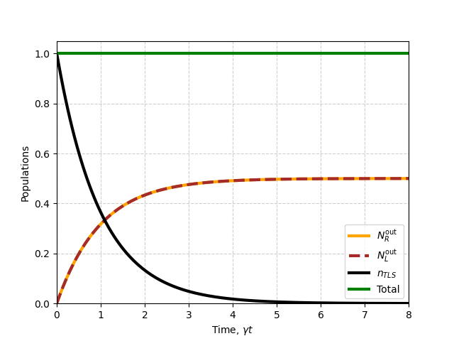
Example plot containing, * Integrated photon flux traveling to the right * Integrated photon flux traveling to the left * TLS population * Conservation check (for one excitation it should be 1)

"""Plotting the results"""
plt.plot(tlist,np.real(net_flux_r),linewidth = 3,color = 'orange',linestyle='-',label=r'$N^{\rm out}_{R}$') # Photons propagating to the right channel
plt.plot(tlist,np.real(net_flux_l),linewidth = 3,color = 'brown',linestyle='--',label=r'$N^{\rm out}_{L}$') # Photons propagating to the left channel
plt.plot(tlist,np.real(tls_pop),linewidth = 3, color = 'k',linestyle='-',label=r'$n_{TLS}$') # TLS population
plt.plot(tlist,np.real(total_quanta),linewidth = 3,color = 'g',linestyle='-',label='Total') # Conservation check (for one excitation it should be 1)
plt.legend()
plt.xlabel(r'Time, $\gamma t$')
plt.ylabel('Populations')
plt.grid(True, linestyle='--', alpha=0.6)
plt.ylim([0.,1.05])
plt.xlim([0.,tmax])
plt.show()

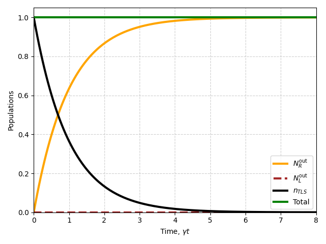
Right Chiral Solution

Similar example but now for a chiral TLS with an updated coupling to be coupled only to the right channel

Update the simulation coupling

gamma_l,gamma_r=qmps.coupling('chiral_r',gamma=1)

input_params.gamma_l=gamma_l
input_params.gamma_r=gamma_r

Update Hamiltonian with new coupling

hm=qmps.hamiltonian_1tls(input_params)

Calculate the time evolution

"""Calculate time evolution of the system"""
bins = qmps.t_evol_mar(hm,sys_initial_state,wg_initial_state,input_params)

Calculate the observables

"""Calculate population dynamics"""
tls_pop_ch = qmps.single_time_expectation(bins.system_states, tls_pop_op)
photon_fluxes_ch = qmps.single_time_expectation(bins.output_field_states, photon_pop_ops)

net_fluxes = np.cumsum(photon_fluxes_ch, axis=1) * delta_t
total_quanta_ch = tls_pop_ch + np.sum(net_fluxes, axis=0)

Plot the results

"""Plotting the results"""
plt.plot(tlist,np.real(net_fluxes[1]),linewidth = 3,color = 'orange',linestyle='-',label=r'$N^{\rm out}_{R}$') # Photons propagating to the right channel
plt.plot(tlist,np.real(net_fluxes[0]),linewidth = 3,color = 'brown',linestyle='--',label=r'$N^{\rm out}_{L}$') # Photons propagating to the left channel
plt.plot(tlist,np.real(tls_pop_ch),linewidth = 3, color = 'k',linestyle='-',label=r'$n_{TLS}$') # TLS population
plt.plot(tlist,np.real(total_quanta_ch),linewidth = 3,color = 'g',linestyle='-',label='Total') # Conservation check (for one excitation it should be 1)
plt.legend()
plt.xlabel(r'Time, $\gamma t$')
plt.ylabel('Populations')
plt.grid(True, linestyle='--', alpha=0.6)
plt.ylim([0.,1.05])
plt.xlim([0.,tmax])
plt.tight_layout()
plt.show()